Can the model reproduce the lynx–hare cycle
The most famous ecological cycle in the world is the hare and the lynx in Canada: roughly every 10 years their numbers swing by a factor of tens. I tested whether my toy ecosystem could reproduce it. The period — yes, easily. Everything else — no.
A pilot of calibrating the model against real data. The question is not “is this true about hares” but “can we honestly compare a model with a real series and see where it breaks”. October 2026.
The model is the ecosystem from iteration 1, without evolution: herbivores and predators wander randomly and eat when they can.
In short
- A ~10-year cycle is easy to get. But it is a weak test: the period is set almost entirely by a free knob, “how many model steps make one year”.
- The lynx lag is not reproduced. In the data the lynx peak trails the hare peak by ~1.5 years. In the model it is 2.5–3 years, and parameter fitting barely moves it.
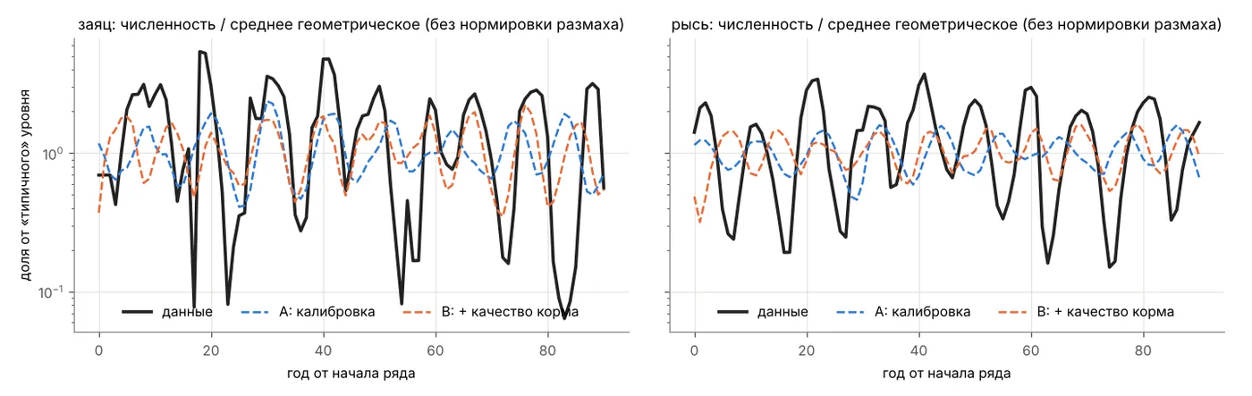
- The swings are 2–3 times smaller than in reality. The real hare varies about 40-fold from trough to peak; the model, 3–5-fold.
- The shape of the cycle matched, but almost any cycling model gives that near-sinusoidal shape. Weak confirmation.
- Bottom line: there is a cycle with the right period, but not the real lynx–hare cycle. The two informative metrics — lag and amplitude — did not match.
Data
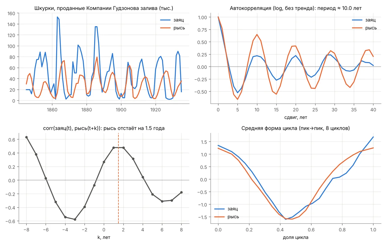
The number of snowshoe hare and Canada lynx pelts sold by trappers to the Hudson’s Bay Company in 1845–1935. The numbers were not edited. A lynx series from the Mackenzie River (1821–1934) was used to check the period independently.
| What the data show | Value |
|---|---|
| Cycle period | ~10 years (Mackenzie: 9.7) |
| How far the lynx trails the hare | 1.5 years = 0.15 of a cycle |
| Swing, hare / lynx | ≈ 40 / 14-fold from trough to peak |
| Share of the cycle spent growing | about half for both |
The hare series is noticeably less regular than the lynx series — a known feature of the pelt record.
How I compared
- Shape is compared, not absolute numbers. Pelts are not population counts, so the metrics are period, lynx lag, amplitude and cycle shape.
- Tolerances come from the data themselves: how much each metric varies across 45-year windows of the real series. “Matched” means the difference is within two such spreads.
- Only period and lag were fitted. Nine model parameters (plant growth, hare metabolism and mortality, lynx hunting and mortality, steps per year) were fitted with the CMA-ES algorithm.
- Amplitude and shape were held out. If the model is right, they should match on their own.
- Guarding against fitting noise: the 20 best candidates were rechecked on 8 fresh random seeds. All numbers below come from those.
Before calibration: with iteration 1 parameters the lynx goes extinct in every run. Of 96 random parameter sets, both populations survive in 31 and a clear cycle appears in 5. In all five the lynx lags by 0.28–0.32 of a cycle.
The best result
Shown is a run of median, not best, quality. The series are normalised and the start of the simulation is shifted to align its phase with the hare. There is no other fitting in the picture.
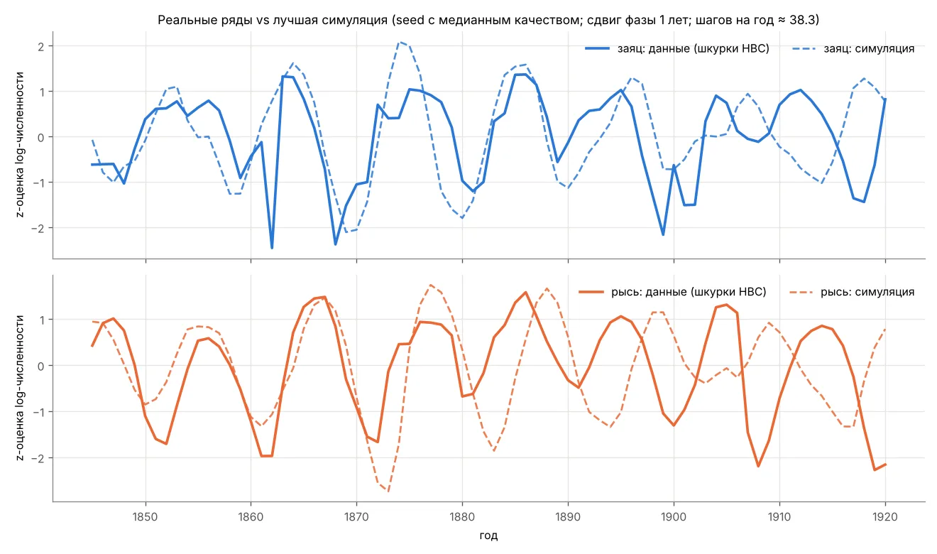
Careful: normalisation hides the main failure. Without it you can see how much deeper the real cycle is:
An attempted fix: worse food when hares are many
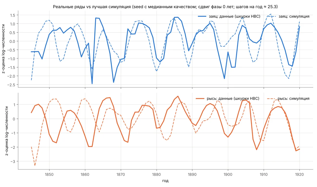
The classic explanation for the short lag is that hares start declining before the lynx peak, because they eat out their food and plants defend themselves. I added a simple feedback: when hares are abundant, food quality drops with a delay, and a hare gets less energy from eating. This is calibration B.
- The fit chose a weak effect: food quality varies only between 0.88 and 0.92.
- It cannot be stronger: hares underfeed and die out, and the lynx follows.
- The lag improved only slightly (0.27 → 0.25 of a cycle); the swing did not grow, and the cycle became less regular.
- Some candidates gave a lag of ~0.20, but the cycle nearly vanished in them. In this model a short lag is bought at the cost of destroying the cycle.
Metrics summary
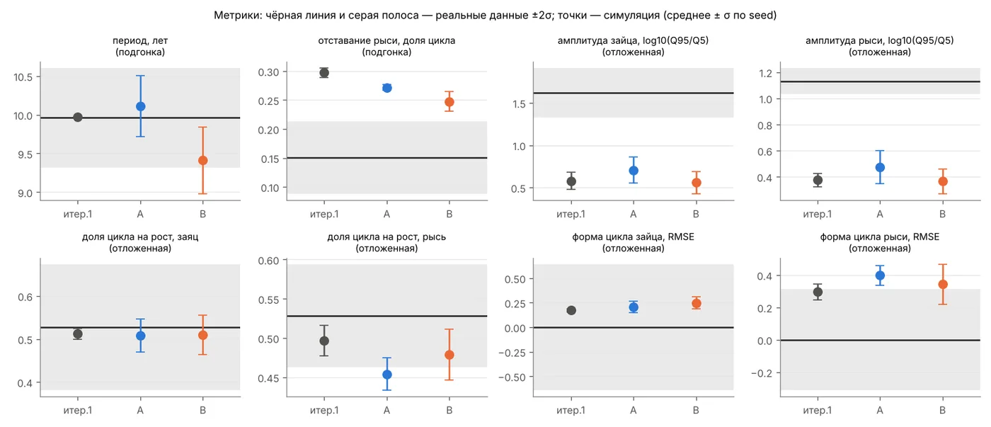
| Metric | Data | A | B |
|---|---|---|---|
| period, years (fitted) | 9.96 | 10.11 ✔ | 9.41 ✔ |
| lynx lag, share of cycle (fitted) | 0.15 | 0.27 ✘ | 0.25 ✘ |
| hare amplitude (held out) | 1.62 | 0.71 ✘ | 0.56 ✘ |
| lynx amplitude (held out) | 1.13 | 0.47 ✘ | 0.36 ✘ |
| share of cycle growing, hare (held out) | 0.53 | 0.51 ✔ | 0.51 ✔ |
| lynx cycle shape (held out) | — | ✘ | ✘ |
Amplitude is log10 of the ratio of high to low levels; 1.62 means roughly 40-fold. ✔ — the difference is within two spreads of the data. B’s improvement over A is small and statistically shaky, even though B has two more parameters.
Why it most likely does not match
The model’s predator reproduces “from its energy reserve” and responds to prey with inertia, as in the classic Lotka–Volterra model. Such a system hits a lag of about a quarter cycle. In reality hares apparently start falling before the lynx peak: because of food, stress, other predators. The limitation looks structural, not a matter of parameters.
The small amplitude is probably due to the world being small and spatial: hundreds of individuals on a 56 × 56 grid, where chance and local encounters damp large swings.
One more hint: at the fitted time scale a hare in the model lives 4–7 “years” without hunger or predators, while a real snowshoe hare lives 1–2 years. The model cannot produce a fast prey population.
How well-determined the parameters are
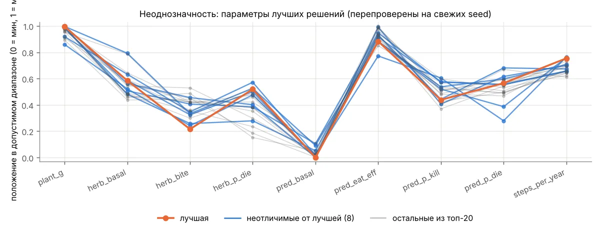
Poorly. In calibration A, 8 of the 20 best candidates are indistinguishable, and lynx mortality varies across them by 25–40%. In B, 11 of 20 are indistinguishable, and lynx metabolism varies sixfold. By period and lag, B’s parameters are almost undetermined. And this is a lower bound: all candidates come from one fitting run.
Several parameters hit the edges of the allowed range (plant growth at the maximum, lynx metabolism at the minimum). That signals not precision but a model “straining” beyond the reasonable. The bounds were deliberately not widened: fitting with exotic values would make the result meaningless.
Limitations. The data are pelt counts, not population: they depend on fur prices, trapping effort and the company’s logistics. Lag is exactly the metric trade can distort most. One series, about 9 cycles, with noisy metrics of its own. The period fits almost trivially, so matching it is a weak achievement. The model is small and spatial; world size was not calibrated. The structural variant B is a single crude one (one food quality for the whole world). A global optimum of the fit is not guaranteed, although none of the 96 random cycling candidates had a lag below 0.28.
What’s next
- The reverse check: fit amplitude and shape, test the lag.
- A different structure: food regrows with a local delay, cell by cell; a larger or less “spatial” world.
- An observation model: pelts = f(population, trapping effort) with its own noise. Needed before paleodata, where “proxy ≠ population” is even stronger.
- An independent check on the Mackenzie series: lynx period and amplitude.
Code, data and all charts are in the evo-brain-sim repository (calibration folder). To discuss, message me on Telegram.